The Explanation: How does this project worK?
"To what degree can a neighborhood's crime rates be
predicted with economic factors?"
(which is what this summary represents:)
Can Crime per Capita (in a zipcode) can be predicted with these economic factors below?
- Zipcode-based Economic factor 1: % of Population Below Poverty Level
- Zipcode-based Economic factor 2: Median Household Income
- Zipcode-based Economic factor 3: Median Rent price of dwellings
The anwser is YES, quite strongly-- with 70-80% confidence, depending on crime type, in Austin, TX
How you ask? Jump to how, in section: "The Results"
I aggregated data from, and data-engineered, the following datasets:
The result is cleansed data, aggregated into following table.
Data table used in the model. Scroll Horizontally & Vertically to see all data
| # |
zipcode |
SqMtrs |
SqKm |
PopulationBelowPovertyLevel |
MedianHouseholdIncome |
Unemployment |
MedianRent |
population |
assault |
burglary |
homicide |
rape |
robbery |
theft |
assault_perCapita |
burglary_perCapita |
homicide_perCapita |
rape_perCapita |
robbery_perCapita |
theft_perCapita |
totalCrimes |
totalCrimesPerCapita |
|---|
| 1 |
78617 |
179810277 |
179.810277 |
18 |
43957 |
15 |
1041 |
19553 |
14 |
48 |
0 |
10 |
12 |
190 |
0.000716002659438449 |
0.00245486626093183 |
0 |
0.000511430471027464 |
0.000613716565232957 |
0.00971717894952181 |
274 |
0.0140131949061525 |
| 2 |
78701 |
4218139 |
4.218139 |
20 |
68152 |
9 |
1590 |
5642 |
84 |
83 |
1 |
34 |
58 |
1776 |
0.0148883374689826 |
0.0147110953562566 |
0.000177242112725984 |
0.00602623183268345 |
0.0102800425381071 |
0.314781992201347 |
2036 |
0.360864941510103 |
| 3 |
78702 |
12944540 |
12.94454 |
33 |
34734 |
11 |
766 |
21032 |
120 |
374 |
2 |
22 |
75 |
1603 |
0.00570559147965006 |
0.0177824267782427 |
9.5093191327501e-05 |
0.00104602510460251 |
0.00356599467478129 |
0.076217192848992 |
2196 |
0.104412324077596 |
| 4 |
78703 |
14436159 |
14.436159 |
10 |
92606 |
4 |
1183 |
19873 |
9 |
76 |
0 |
3 |
7 |
565 |
0.000452875761082876 |
0.00382428420469984 |
0 |
0.000150958587027625 |
0.000352236703064459 |
0.0284305338902028 |
660 |
0.0332108891460776 |
| 5 |
78704 |
22503945 |
22.503945 |
21 |
50248 |
7 |
940 |
41709 |
96 |
318 |
2 |
22 |
34 |
2243 |
0.00230166151190391 |
0.00762425375818169 |
4.7951281497998e-05 |
0.000527464096477978 |
0.000815171785465967 |
0.0537773622000048 |
2715 |
0.0650938646335323 |
| 6 |
78705 |
5686651 |
5.686651 |
66 |
11917 |
14 |
1088 |
30532 |
31 |
133 |
0 |
32 |
18 |
924 |
0.00101532818026988 |
0.00435608541857723 |
0 |
0.00104808070221407 |
0.000589545394995415 |
0.0302633302764313 |
1138 |
0.0372723699724879 |
| 7 |
78717 |
33415021 |
33.415021 |
3 |
93305 |
5 |
1018 |
23514 |
10 |
56 |
0 |
1 |
0 |
190 |
0.000425278557455133 |
0.00238155992174875 |
0 |
4.25278557455133e-05 |
0 |
0.00808029259164753 |
257 |
0.0109296589265969 |
| 8 |
78721 |
9588238 |
9.588238 |
32 |
32131 |
16 |
870 |
11178 |
67 |
146 |
0 |
9 |
23 |
394 |
0.00599391662193595 |
0.0130613705492933 |
0 |
0.000805152979066023 |
0.00205761316872428 |
0.0352478081946681 |
639 |
0.0571658615136876 |
| 9 |
78722 |
3919536 |
3.919536 |
19 |
44917 |
8 |
930 |
5973 |
12 |
57 |
0 |
3 |
10 |
265 |
0.00200904068307383 |
0.0095429432446007 |
0 |
0.000502260170768458 |
0.00167420056922819 |
0.0443663150845471 |
347 |
0.0580947597522183 |
| 10 |
78723 |
17979293 |
17.979293 |
29 |
41869 |
10 |
817 |
30999 |
149 |
330 |
4 |
42 |
51 |
1507 |
0.00480660666473112 |
0.0106455046936998 |
0.000129036420529694 |
0.00135488241556179 |
0.00164521436175361 |
0.0486144714345624 |
2083 |
0.0671957159908384 |
| 11 |
78724 |
63858033 |
63.858033 |
38 |
35711 |
8 |
962 |
21677 |
48 |
127 |
0 |
18 |
17 |
327 |
0.00221432855099875 |
0.0058587442911842 |
0 |
0.000830373206624533 |
0.000784241361812059 |
0.015085113253679 |
537 |
0.0247728006642986 |
| 12 |
78726 |
28204228 |
28.204228 |
9 |
66096 |
4 |
1050 |
12482 |
6 |
16 |
0 |
4 |
2 |
176 |
0.000480692196763339 |
0.00128184585803557 |
0 |
0.000320461464508893 |
0.000160230732254446 |
0.0141003044383913 |
204 |
0.0163435346899535 |
| 13 |
78727 |
22190828 |
22.190828 |
11 |
65687 |
6 |
1050 |
28461 |
22 |
78 |
3 |
9 |
5 |
415 |
0.000772987597062647 |
0.00274059238958575 |
0.000105407399599452 |
0.000316222198798356 |
0.00017567899933242 |
0.0145813569445908 |
532 |
0.0186922455289695 |
| 14 |
78728 |
21004795 |
21.004795 |
14 |
47405 |
6 |
901 |
20939 |
0 |
2 |
0 |
0 |
0 |
6 |
0 |
9.5515545154974e-05 |
0 |
0 |
0 |
0.000286546635464922 |
8 |
0.000382062180619896 |
| 15 |
78729 |
23786144 |
23.786144 |
8 |
57358 |
7 |
1008 |
28228 |
22 |
78 |
0 |
4 |
8 |
357 |
0.000779368003400879 |
0.00276321383023948 |
0 |
0.000141703273345614 |
0.000283406546691229 |
0.0126470171460961 |
469 |
0.0166147087997733 |
| 16 |
78730 |
37840281 |
37.840281 |
4 |
119573 |
3 |
1106 |
8312 |
3 |
8 |
0 |
2 |
0 |
38 |
0.000360923965351299 |
0.000962463907603465 |
0 |
0.000240615976900866 |
0 |
0.00457170356111646 |
51 |
0.00613570741097209 |
| 17 |
78731 |
22412156 |
22.412156 |
9 |
78265 |
4 |
1016 |
24716 |
12 |
83 |
0 |
7 |
4 |
421 |
0.000485515455575336 |
0.00335814856772941 |
0 |
0.000283217349085613 |
0.000161838485191779 |
0.0170335005664347 |
527 |
0.0213222204240168 |
| 18 |
78732 |
34465142 |
34.465142 |
3 |
127726 |
5 |
1688 |
14307 |
0 |
0 |
0 |
0 |
0 |
3 |
0 |
0 |
0 |
0 |
0 |
0.000209687565527364 |
3 |
0.000209687565527364 |
| 19 |
78735 |
53215463 |
53.215463 |
6 |
74571 |
4 |
1122 |
16882 |
11 |
50 |
0 |
2 |
2 |
215 |
0.000651581566165146 |
0.00296173439165976 |
0 |
0.00011846937566639 |
0.00011846937566639 |
0.0127354578841369 |
280 |
0.0165857125932946 |
| 20 |
78739 |
29628564 |
29.628564 |
1 |
126525 |
4 |
2000 |
16911 |
1 |
13 |
0 |
1 |
0 |
118 |
5.91331086275206e-05 |
0.000768730412157767 |
0 |
5.91331086275206e-05 |
0 |
0.00697770681804743 |
133 |
0.00786470344746023 |
| 21 |
78741 |
19660250 |
19.66025 |
40 |
30183 |
9 |
835 |
48246 |
225 |
598 |
1 |
54 |
130 |
2386 |
0.00466359905484392 |
0.0123948099324296 |
2.07271069104174e-05 |
0.00111926377316254 |
0.00269452389835427 |
0.049454877088256 |
3394 |
0.0703478008539568 |
| 22 |
78742 |
14852580 |
14.85258 |
37 |
34076 |
11 |
639 |
901 |
4 |
11 |
0 |
2 |
0 |
29 |
0.00443951165371809 |
0.0122086570477248 |
0 |
0.00221975582685905 |
0 |
0.0321864594894562 |
46 |
0.051054384017758 |
| 23 |
78744 |
55439912 |
55.439912 |
26 |
41056 |
9 |
946 |
43452 |
135 |
407 |
4 |
35 |
51 |
1563 |
0.00310687655343828 |
0.00936665746110651 |
9.20556015833563e-05 |
0.000805486513854368 |
0.00117370892018779 |
0.0359707263186965 |
2195 |
0.0505155113688668 |
| 24 |
78745 |
34600328 |
34.600328 |
16 |
49243 |
7 |
990 |
54917 |
120 |
435 |
1 |
34 |
37 |
1950 |
0.00218511572008668 |
0.0079210444853142 |
1.8209297667389e-05 |
0.000619116120691225 |
0.000673744013693392 |
0.0355081304514085 |
2577 |
0.0469253600888614 |
| 25 |
78746 |
58326014 |
58.326014 |
5 |
125327 |
4 |
1221 |
26939 |
6 |
36 |
0 |
2 |
5 |
741 |
0.000222725416682134 |
0.0013363525000928 |
0 |
7.42418055607112e-05 |
0.000185604513901778 |
0.0275065889602435 |
790 |
0.0293255131964809 |
| 26 |
78748 |
32834705 |
32.834705 |
9 |
65889 |
6 |
1095 |
40290 |
48 |
203 |
2 |
13 |
14 |
1270 |
0.00119136262099777 |
0.00503847108463639 |
4.96401092082403e-05 |
0.000322660709853562 |
0.000347480764457682 |
0.0315214693472326 |
1550 |
0.0384710846363862 |
| 27 |
78749 |
26078902 |
26.078902 |
6 |
80956 |
4 |
1150 |
34391 |
26 |
86 |
2 |
6 |
9 |
689 |
0.000756011747259457 |
0.00250065424093513 |
5.8154749789189e-05 |
0.000174464249367567 |
0.000261696374051351 |
0.0200343113023756 |
818 |
0.0237852926637783 |
| 28 |
78750 |
34718029 |
34.718029 |
7 |
75958 |
6 |
1012 |
27119 |
16 |
72 |
2 |
4 |
7 |
308 |
0.000589992256351635 |
0.00265496515358236 |
7.37490320439544e-05 |
0.000147498064087909 |
0.00025812161215384 |
0.011357350934769 |
409 |
0.0150816770529887 |
| 29 |
78751 |
6211942 |
6.211942 |
26 |
38624 |
9 |
865 |
14340 |
22 |
100 |
0 |
8 |
11 |
785 |
0.00153417015341702 |
0.00697350069735007 |
0 |
0.000557880055788006 |
0.000767085076708508 |
0.054741980474198 |
926 |
0.0645746164574616 |
| 30 |
78752 |
8657144 |
8.657144 |
32 |
33271 |
9 |
752 |
17170 |
101 |
162 |
0 |
23 |
49 |
986 |
0.00588235294117647 |
0.00943506115317414 |
0 |
0.00133954571927781 |
0.00285381479324403 |
0.0574257425742574 |
1321 |
0.0769365171811299 |
| 31 |
78753 |
28417686 |
28.417686 |
26 |
39593 |
9 |
826 |
52384 |
184 |
440 |
4 |
58 |
111 |
3138 |
0.00351252290775809 |
0.00839951130116066 |
7.63591936469151e-05 |
0.00110720830788027 |
0.00211896762370189 |
0.0599037874160049 |
3935 |
0.0751183567501527 |
| 32 |
78754 |
34419093 |
34.419093 |
11 |
53274 |
9 |
969 |
13570 |
21 |
94 |
0 |
1 |
2 |
339 |
0.00154753131908622 |
0.00692704495210022 |
0 |
7.36919675755343e-05 |
0.000147383935151069 |
0.0249815770081061 |
457 |
0.0336772291820192 |
| 33 |
78756 |
4329297 |
4.329297 |
9 |
59685 |
4 |
888 |
8060 |
8 |
76 |
0 |
1 |
3 |
267 |
0.000992555831265509 |
0.00942928039702233 |
0 |
0.000124069478908189 |
0.000372208436724566 |
0.0331265508684863 |
355 |
0.0440446650124069 |
| 34 |
78757 |
12732626 |
12.732626 |
16 |
55156 |
6 |
895 |
22718 |
21 |
189 |
2 |
13 |
15 |
858 |
0.000924377145875517 |
0.00831939431287966 |
8.80359186548112e-05 |
0.000572233471256273 |
0.000660269389911084 |
0.037767409102914 |
1098 |
0.0483317193414913 |
| 35 |
78758 |
24052435 |
24.052435 |
24 |
41792 |
10 |
898 |
45105 |
155 |
412 |
0 |
36 |
79 |
2144 |
0.00343642611683849 |
0.00913424232346747 |
0 |
0.000798137678749584 |
0.00175146879503381 |
0.047533532867753 |
2826 |
0.0626538077818424 |
| 36 |
78759 |
36065378 |
36.065378 |
7 |
65672 |
7 |
962 |
39850 |
31 |
156 |
1 |
9 |
15 |
1345 |
0.000777917189460477 |
0.00391468005018821 |
2.50941028858218e-05 |
0.000225846925972396 |
0.000376411543287328 |
0.0337515683814304 |
1557 |
0.0390715181932246 |
From here-- with our .csv file of data, we are ready to put the multilinear
regression model to work.
The process:
I collected datasets for zipcodes in Austin showing the economic indicators mentioned above
for each zipcode (the median income, median rent, and percentage of residents in poverty for 36
Austin, Texas zipcodes). I then cross-referenced these zipcodes with a dataset of about 40,000
crimes that occured in Austin in a particular year. I excluded all zipcodes except those for which
I had data for both economic indicators and crimes. I then counted up crimes per category (6
categories total, after similfying category names: Assault, Burglary, Robbery, Theft, Homicide,
and Rape), per zipcode. With these two datasets showing economic & crime data for particular
zipdoes, we are able to produce an equation showing the degree of confidence with which we can
predict rates of crime based on the chosen economic indicators.
The results:
According to coefficient of determination for the various models, we can say that about
70%-80% of the variability in these crimes—Assault, Burglary, and Robbery (for the zip
codes examined) can be explained by the variability in the selected economic indicators.
That's a pretty strong connection which means that these three types of crimes can be relatively
well explained based on these three economic indicators (income, rent, and % of population below
poverty)! Based on this study, the other types of crimes examined (homicide and rape) cannot be
reliably predicted based on economic indicators– this means they're less determined by
economic health of a neighborhood, and more by other unknown/non-analyzed factors.
The ultimate purpose of the project was to create a statistical model from the
"training" dataset – i.e. a model that explains the data – and then to test the
"test" dataset upon the training model, to check how well the model can be used to predict crime
rates based on the economic factors studied.
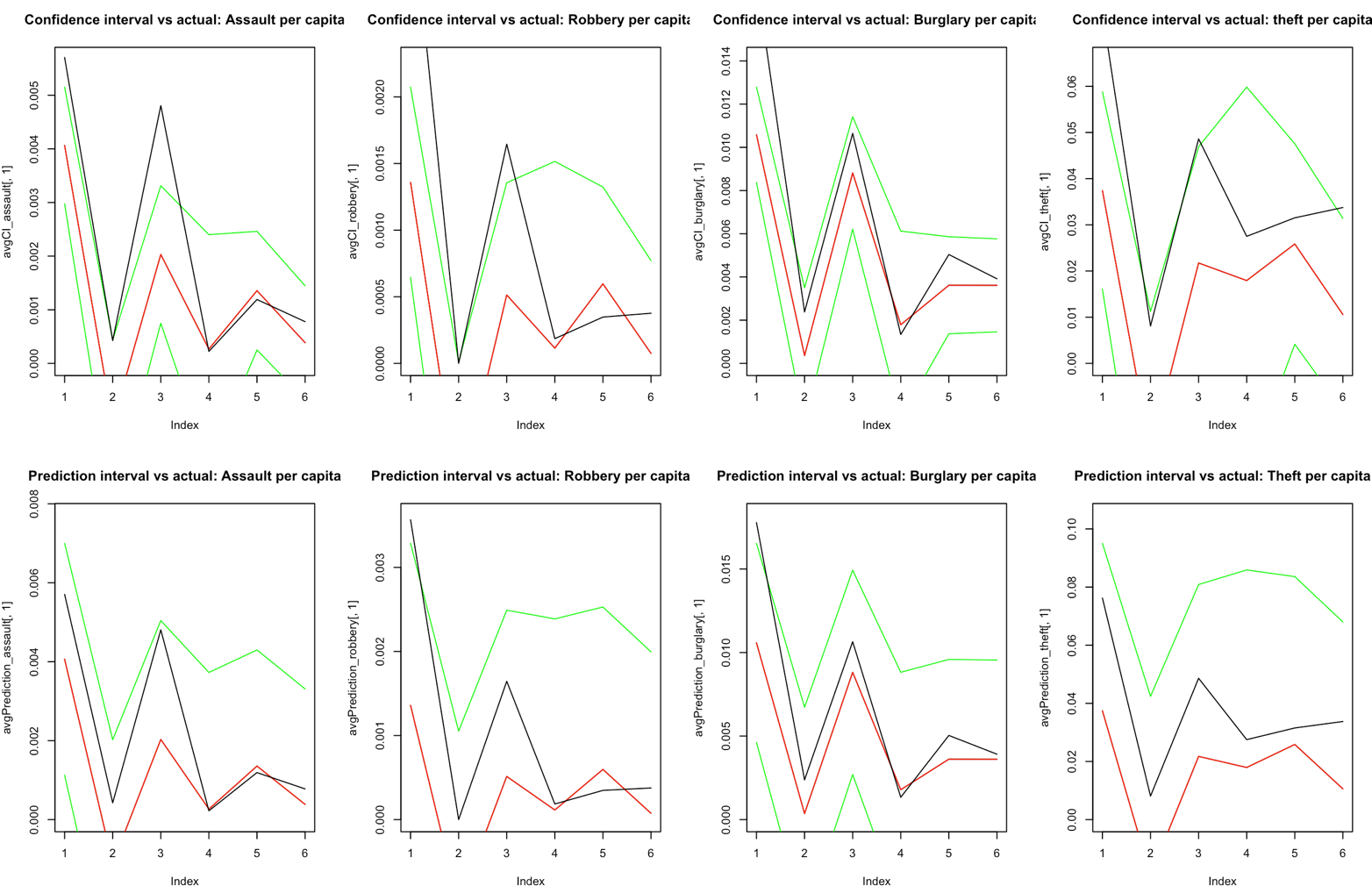
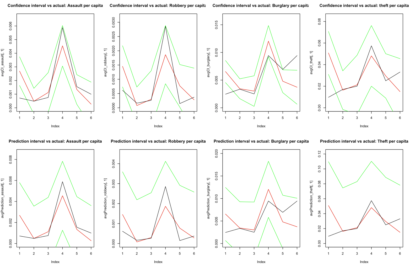
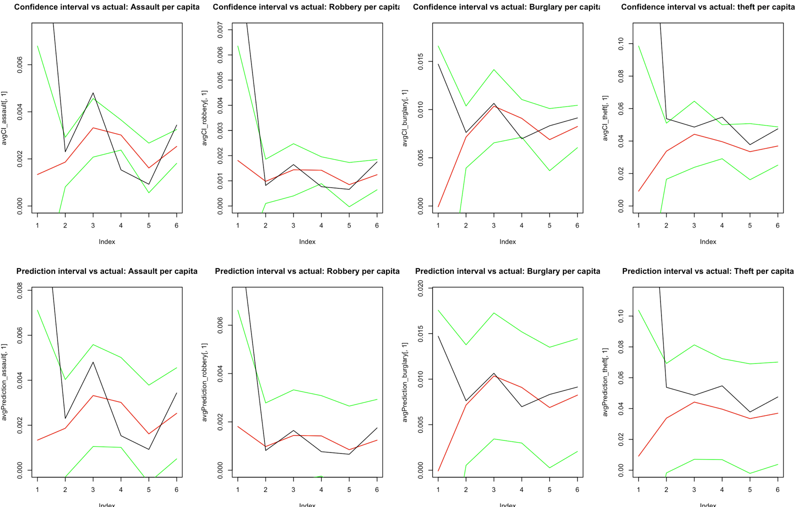
In the statistical charts-- the colorful lines at the top of this page--
we can visualize how well the model
predicts crime based on the economic factor inputs from the training dataset. The green
lines show the boundaries of a 95% confidence interval (we can be "95% certain" that this
interval contains the true mean of the population, which we use the data in the test group to
simulate a sample of.), with the redline being the predicted average. The black
line represents the actual test data used. As you can see, the green lines capture the
majority of the datapoints from the test data, showing that this model (using economic data to
explain crimes) does quite a good job of some of these predicting specific crimes (assault,
robbery, and especially burglary).
I programmed the project for my two other teammates, who provided guidance, feedback, and
ideation, and the final script can be viewed here.
Why do I enjoy statistical analysis?
I enjoy statistical analysis because it is a creative, fun, puzzle-solving way of
thinking which allows us to explain the world through data in meaningful, measurable
ways.
Throughout this particular statistics course ("Advanced Statistical Methods"), I
noticed my thought processes changing. I noticed this especially while working on my statistics
project, and for me, I think I really changed between the day I walked into the class, and the
day class ended. I realized then that I had began to think more analytically and from a more
data-driven, input-output, and equation-based perspective. Crafting equations from data is
solving a puzzle– a puzzle where you can produce real and fascinating answers from
apparently unrelated datasets! It's quite fun once you get into it!
In addition to changing the way you think, and having fun analyzing a real life puzzle...
practicing statistics via scripting will improve your programming abilities! Learning R really
helped me become a better programmer because before I could start playing with data, I spent
plenty of time learning R's data types and data structures, which was useful when it came time
to produce an analysis project and is applicable to programming.
I really like statistics in general for the contribution that the multivariate analysis makes
when analyzing any kind of ideas, really. It is quite handy for empirically analyzing all sorts
of ideas: whether business decisions, scientific & engineering projects, economic theories, or
policy arguments. Being able to formulate an equation or model based on data is a skill in its
own right.
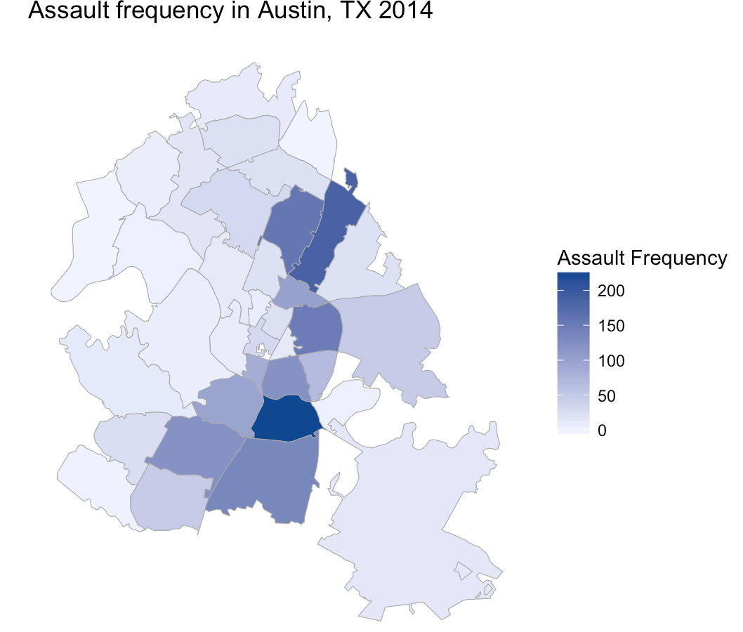
One of my favorite data visualizations is the "choropleth map", i.e. heatmap.
Here's a choropleth map of Assault frequency for zipcodes in Austin, TX (data is annual
assaults reported in 2014).